I’ve started learning Julia. It has been awhile since I taught myself a new language. I’ve been doing a combination of two things. 1) Working my way through Think Julia: How to Think Like a Computer Scientist. 2) I’ve been trying to implement a random forest model using an abalone data set I downloaded for another project. Between these 2 methods, I’ve picked up a few things. I’m going to work through a few basic ideas here.
A little bit of set up before I get into this. I’m running these Julia code chunks in an Rmarkdown file (because that’s why way my website is set up). To get them to work you need to install the JuliaCall package & add a few extra lines of code to your setup code chunk. I’ve left the code chunk visible so you can see how I made this work. Also, you need to have RCall installed in Julia!
library(JuliaCall)
julia_path = "/Applications/Julia-1.7.app/Contents/Resources/julia/bin"
julia_setup(julia_path)

knitr::opts_chunk$set(echo = TRUE)
Let’s get into it! You can get the data file I used here. abalone.data is the file we are going to be working with. Similar to R, we start by loading the packages we want to use. I prefer to set a path variable BASE_DIR as a standardized prefix for data files & any eventual output files.
using DataFrames
using CSV

# set base directory variable
BASE_DIR = "/Users/sarah/Documents/learn_Julia/random_forest/data";

println(BASE_DIR)
## /Users/sarah/Documents/learn_Julia/random_forest/data
Tip: using println() instead of print adds a new line to the end of whatever you print.
Now that we’ve set our path, let’s read in our file. There are a couple different ways to do that. Isn’t there always?! I chose this way because it was the easiest for me to understand. Also, this dataset is relatively small so we aren’t very worried about it taking too long to load.
The string() function concatenates our BASE_DIR variable with the file name. By specifying DataFrame, we can save our newly read in file as a data frame object immediately. We set the delimiter to , using delim = ",". We tell the CSV.read() function that our file has no hdear by using header = false.
We’ll use first() to take a quick look at our data frame before we move on.
dat = CSV.read(string(BASE_DIR, "/abalone.data"), DataFrame; delim = ",", header = false);

first(dat, 5)
## 5×9 DataFrame
##  Row │ Column1  Column2  Column3  Column4  Column5  Column6  Column7  Column8  ⋯
##      │ String1  Float64  Float64  Float64  Float64  Float64  Float64  Float64  ⋯
## ─────┼──────────────────────────────────────────────────────────────────────────
##    1 │ M          0.455    0.365    0.095   0.514    0.2245   0.101     0.15   ⋯
##    2 │ M          0.35     0.265    0.09    0.2255   0.0995   0.0485    0.07
##    3 │ F          0.53     0.42     0.135   0.677    0.2565   0.1415    0.21
##    4 │ M          0.44     0.365    0.125   0.516    0.2155   0.114     0.155
##    5 │ I          0.33     0.255    0.08    0.205    0.0895   0.0395    0.055  ⋯
##                                                                 1 column omitted
Tip: If you’re working in Visual Studio, etc, you don’t have to use a semicolon at the end of each line. I’m doing it here to stop the output from automatically printing in R markdown.
So now that we have our data frame. Let’s rename our columns to something useful! We use rename() to set the names of each column. Then use first() to look at our handiwork.
rename!(dat, [:Sex, :Length, :Diameter, :Height, :Whole_Weight, :Shucked_Weight, :Viscera_Weight, :Shell_Weight, :Rings]);

first(dat, 5)
## 5×9 DataFrame
##  Row │ Sex      Length   Diameter  Height   Whole_Weight  Shucked_Weight  Visc ⋯
##      │ String1  Float64  Float64   Float64  Float64       Float64         Floa ⋯
## ─────┼──────────────────────────────────────────────────────────────────────────
##    1 │ M          0.455     0.365    0.095        0.514           0.2245       ⋯
##    2 │ M          0.35      0.265    0.09         0.2255          0.0995
##    3 │ F          0.53      0.42     0.135        0.677           0.2565
##    4 │ M          0.44      0.365    0.125        0.516           0.2155
##    5 │ I          0.33      0.255    0.08         0.205           0.0895       ⋯
##                                                                3 columns omitted
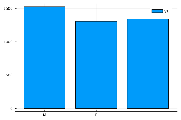
Looks good. I’d like to learn a bit more about the data in my data frame. First, we need to add the StatsBase package. I’m going to use countmap() to find the count of each sex. Our data has 3 sexes: M (male), F (female), & I (infant).
using StatsBase

sex_count_dat = countmap(dat.Sex)
## Dict{String1, Int64} with 3 entries:
##   "I" => 1342
##   "M" => 1528
##   "F" => 1307
That’s informative but let’s plot it to get a better look! First, I’m going to make a list of the values I want on the tick marks in the specified order. Next I’ll use bar to make the plot, using the xticks option to set my tick mark labels.
using StatsPlots

s = ["M", "F", "I"];
bar((x -> sex_count_dat[x]).(s), xticks = (1:3, s))

I’m going to stop here for now! This is definitely a very good start!
Possibly helpful side note Getting Julia to render these plots using R markdown required a couple extra steps. My original Julia installation was 1.6 using the .dmg file provided by the Julia Org website. I wanted to upgrade to 1.7. I installed it using brew install. I ran into an error I couldn’t figure out. I uninstalled v1.7 using brew & then did a new installation from here. Then I ran into a new error could not load library "libjulia.1.dylib". To solve this, I created a symlink from the directory that Julia was looking in to the directory this file was actually in. That seems to have sovled my problem for now! Probably could’ve not spent 3 hours debugging this if I’d just done the symlink thing to begin with!
Also, I had to run brew reinstall icu4c in the terminal to get blogdown::hugo_build() to work. It’s been so long since I’ve done a blog post that I’m not even sure what that’s about.
Hope you found this helpful! If you have any questions/comments/concerns/feedback, I’d love to hear from you! Feel free to reach out to me on Twitter.